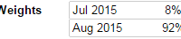
Summary High Contango Is Not a Reflection of Free Market Failure. High Contango Is Your Best Investment Friend. 2011 AAA Downgrade of US Treasuries Lead to The Low Volatility Regime of the S&P 500. VXX/XIV disproving efficient markets. How can a product go up or down EVERY year?! Contango should narrow if efficient market. A couple of days ago I received this tweet from one of my followers on Twitter. While the question is very valid, it belies a common misunderstanding about the two biggest vehicles used to trade volatility – The iPath S&P 500 VIX Short-Term Futures ETN (NYSEARCA: VXX ) and the VelocityShares Daily Inverse VIX Short-Term ETN (NASDAQ: XIV ). In this article, I will try to shed light on the inner workings of VXX and XIV and explain why their behavior has nothing to do with market efficiency and some to do with official government policy and even more to do with the AAA downgrade episode. The Search for the Perfect Trading Vehicle for Volatility VXX has about $800 million in AUM with $950 million trading daily. VXX was launched in January 30th, 2009. It has now been around 6+ years. XIV has about $850 million AUM. The XIV arrived on November 30th, 2010 and has been around for nearly 5 years. XIV and VXX are exact opposites of each other with the VXX going up a certain amount when the VIX goes up that day and XIV going down a similar amount. However, it is important to realize that VXX and XIV do not track the VIX exactly. What they track will be discussed further down. There exists this unfulfilled desire amongst traders of the S&P 500 index and related option and futures instruments to have the perfect hedging vehicle that will eliminate all the risk from their trading endeavors. I mean who doesn’t want that? Buy the VIX at the top of the market, may be put 5% into spot VIX vehicle. Market goes down 5%, VIX goes up 60-70%, no money, no love lost. You get to keep your clients and your money with minimal work. When things go up, make money. When things go down, stay the same. Never lose money, always in the money. Live happily ever after. Unfortunately in the real world, risk exists and risk is forever. There is always a Damoclean sword hanging over your investments. Things can go bad at any moment and no amount of financial trickery and innovation will get you rid of that. The best you can do is replace one risk with another less likely risk. There never will be a trading vehicle that exactly matches the spot VIX index at its sub-second calculation interval. We should never forget that the CBOE VIX is a calculation. It is not an asset like a stock or a bond that has buyers and sellers. It is a calculation that tracks something. It is an absolute technological miracle that it can be calculated in close to real-time as it is. It is an insurmountable logistical challenge to have an intra-day futures market that efficiently settles pricing of daily futures on a second or even minute basis. Once you have that intra-day VIX futures market you can power an ETF that will precisely match the VIX. But even having a daily futures market is close to a physical impossibility. You not only need the technical power to do it (which is astounding). You also need the depth of market, wide ranging liquidity and sufficient participation to enable proper pricing. May be that will become a reality in the future, but at present it isn’t. I see some feeble attempts at it, but I don’t see the true effort that is going to make this a reality. Maybe nobody (except some VIX purists) cares. Why? The VXX and XIV are Already Just Perfect Like all original designs, XIV and VXX are very close to achieving ultimate perfection in the goal they set out to achieve – which is provide a vehicle to trade the VIX. The closest you can get to matching spot VIX in reality is by having a futures market where buyers and sellers get to haggle on what the price of the VIX should be. There is one caveat however. There is no way to haggle about the price of the VIX right now because it is a calculation. You already know mathematically what it is. You also know what it was in the past. What you don’t know is how much it will be in the future. That is where the futures market comes in and buyers and sellers can say – hey I think the VIX is going to be this amount in the future. The buyer puts in a bid, the seller puts in an ask and the haggling goes on happily ever after. So if you want to trade the VIX, your best bet is trading the front month future (which I will call VIX1 henceforth). And a lot of professional traders do just that. But the futures markets are not for the faint of heart. A position is $30,000. You need a special account and approval. Access to futures market is generally only available for professional traders or very sophisticated retail investors. The retail investor population is essentially priced out or qualified out of them. But even if you are pro, the VIX is a very volatile animal and you can lose your shirt rather quickly in the futures market especially as the VIX1 future nears it expiration and then must match the VIX more and more. On settlement day VIX1 is always equal to the VIX. But the VIX can go up or down 20% in one day. In the futures market that means bankruptcy. No ETF maker will undertake this kind of risk. They will be out of business on the first VIX spikage. So they have to devise something that is a little less volatile. Enter VIX2 future. The VIX2 future is a little farther in the future and is not so tied into the present day VIX value. So you would buy the VIX2 future and hedge that by selling the VIX1 future. Ok, now we are getting somewhere. This looks like it could be the makings of an ETF that is a little less volatile and won’t make the issuer bankrupt, but at the same does a serviceable job of giving us an instrument tied to the VIX. May be not a 100% match of the VIX, but a match of 50% is better than nothing (remember, prior to 2009, there was absolutely nothing). Well, this is exactly what VXX does! The VXX buys VIX2 futures and sells VIX1 futures on a daily basis. The closer we are to VIX1 expiration, the smaller the amount of VIX1 futures and the larger the amount of VIX2 futures that are traded. The amount is proportional to the time to expiration. The allocation weight inside the VXX/XIV of VIX1 futures is T1/(T1+T2) and for VIX2 futures it is T2/(T1+T2). The daily weights of the VXX and XIV can be found here (TradingVolatility.net -> Data -> VIX Futures page): The XIV does exactly the same, except for it shorts VIX2 and covers VIX1 daily. And this way, the two ETNs try to approximate the VIX, which I think is still the best way to do accomplish this task baring the emergence of daily VIX Futures market. The Importance of Contango Now that we understand how VXX/XIV work, it isn’t unreasonable to come to the conclusion that the price spread between the VIX1 and VIX2 futures is of particular importance. After all these are your buy /sell prices or short/cover prices. So is there anything to know about the VIX1 and VIX2 pricing spread? Well, there sure is! The price spread between VIX1 and VIX2 is called Contango . Mathematically, Contango = (VIX2/VIX1) – 1 and is measured with a percentage. Before we continue on the topic of Contango, let’s take a broader look of the VIX Futures Curve. (click to enlarge) Source: vixcentral.com The futures curve depicted above is the usual distribution of futures prices in the VIX futures market. The VIX index was designed to be mean reverting so by definition any time the VIX trades at levels below the historical average (which is roughly 20), the market anticipates that the VIX will rise in the future to reach that historical average. In fact, if there was an infinite VIX future, it’s value will be the historical average of 19.46. The condition when second month VIX future (VIX2) is higher than the front-month VIX future (VIX1) is called Contango . So when the VIX Futures Curve is in the above formation, it is considered to be in Contango formation. When the situation is reversed and VIX2 is smaller than VIX1, then the VIX Futures Curve is usually in the below formation which is called Backwardation . (click to enlarge) Source: vixcentral.com Wait a second? Why should the VIX futures try to reach its long term average? The answer can be found on the VIX Primer page on CFE VIX Futures site where they explain how to calculate the Fair Value of a VIX Future. I am going to shamelessly reprint their content here: Fair Value of VIX Futures Futures traders are most familiar with the fair value of stock index futures derived from the cost-of carry relationship between the futures and the underlying stock index. Since there is no carry between VIX and a position in VIX futures, the fair value of VIX futures cannot be derived by a similar relationship. Instead the fair value is derived by pricing the forward 30-day variance which underlies the settlement price of VIX futures. The fair value of VIX futures is the square root of this expected variance less an adjustment factor which reflects the concavity of the square root function used to extract volatility from variance. In percentage points, the fair value of VIX futures is: In this expression, Pt is the forward price of de-annualized variance in the 30 days after the futures expiration, and -vart[FT] is the concavity adjustment. The adjustment subtracts the variance of the futures price at expiration, which can also be expressed as the cumulative daily variance of VIX futures from the current date to expiration. Using methods similar to those on which the calculation of VIX is based, the forward price of the 30-day variance can be determined from a synthetic calendar spread of S&P 500 options bracketing the 30 days after the futures expiration. The variance of the futures price can be estimated from historical data on the daily variance of VIX futures. I don’t want to go into deep mathematical analysis here, the end result of that calculation is that a VIX Future contract over the long term tries to reach the average spot VIX value. The farther out in time the future, the closer the fair value will be to the average historical VIX value. The delta between the future price approximation and the average value goes exponentially closer to zero. The flipside of that calculation is that the nearest term VIX future has the largest difference to the long-term average, the second term VIX Future – the second largest difference, the third term VIX Future – the third largest difference, etc. The exponential decline in the delta can be plainly seen in the usual VIX Future Curve formation depicted above (Contango formation). So as a result, you can kind of guess that Contango is usually some healthy percentage not exactly close to 0%. In fact, the VIX spends most of its time declining from elevated levels. While the average VIX is around 20, the VIX has spent 60% of the time below 20 since its inception in 1990. Since the bull market start in 2009 and the beginning of active Central Bank suppression of volatility that percentage is even higher at 65%. Since 2012 once the AAA downgrade episode passed and QE Infinity was announced, the VIX has spent a remarkable 92% of the time below 20! Since the inception of the VIX Futures in 2004, the average Contango between VIX1 and VIX2 has been 5.6%. Since onset of QE Infinity in 2012, Contango has averaged 7.2% High Contango is NOT a Reflection of Free Market Failure Financial markets are very efficient and well priced. In this age of High Frequency Trading, the bid-ask spread is almost zero for most instruments. There is plenty of liquidity out there. A buyer will always find a seller at a price readily quoted in real time. Yes, there have been technical glitches and blowups but technology can and will be fixed over time. However, the markets are also very, very manipulated. Central Banks have the power of the printing press and can overwhelm financial markets with the liquidity available to them. It is critical to understand that it is a core mandate of the Central Banks to suppress volatility . After all, “stable prices” is mandate #2 of the Federal Reserve. The Central Banks do not want the S&P 500 index to go down 50%. In fact, they don’t want it to go down 10%. They want the index to go up or trade in a small range at worst, regardless of fundamental valuation. Stock market panics and large drawdowns have had large spillover effects on the broader economy and in 2000 and 2008 brought about recessions. The FED and other Central Banks want to avoid a repeat of those episodes and as such deploy rarely announced techniques to suppress volatility and honest price discovery. The Bank of Japan, for example, buys stock futures in the open market. Central Banks of other smaller countries also purchase stock futures. In fact, the Chicago Mercantile Exchange (NASDAQ: CME ) has a Central Bank Incentive Program where non-US Central Banks can buy S&P 500 E-mini Equity Index Futures and Options at a discount. Whether that is right or wrong is above my pay grade, the point is that it is happening. However, as much we want to blame the FED for everything, it ultimately is not the FED’s fault that markets have risen non-stop since 2012 with very little volatility. The AAA downgrade episode in 2012 marked a fundamental change in what is perceived as a risk free asset. Prior to 2012, US government treasuries were the de-facto risk free asset featuring a AAA credit rating. Well, US government debt is no longer AAA rated. Not according to the Standard & Poors. However, the S&P 500 is definitely still AAA rated. The S&P 500 features the best of American and international industry with steady earnings and cash flow. If you were Black Rock and had tens of billions to invest, where would you invest? In AA+ US government long-term debt that barely yields 2.5% or the S&P 500 that has a 1.9% dividend yield, usually a 5% expected annual earnings growth and is AAA rated? I think you have seen the answer. Since 2012, every major institutional investor whether it is foreign central banks, college endowments, large asset managers, etc have been pouring money into the S&P500 non stop with no end in sight. So as much as we want to blame the FED for the compression of volatility, the FED is partly to blame. Majority of the blame falls on the divided and dysfunctional US government and Standard & Poors, who for a change, have refused to close their eyes to reality and have assigned the proper credit rating. So high Contango is here to stay until the US government regains its AAA rating. So How Can I Benefit From High Contango? Now that you know that contango has been high and will continue to be high, how do we turn that into investment profits? You can gain an edge in these Central Bank controlled markets by including outperforming volatility products in your portfolio. After all, you do know volatility is being suppressed. What you don’t know is whether companies will continue to increase earnings. You don’t know with certainty if companies can match with earnings, the price assigned to them by the market. In 2015, they have been failing in that regard and as a result the P/E ratio of the S&P 500 has continued to grind higher and higher. However, as valuations soar, it gets harder and harder for individual stocks to appreciate significantly on a percentage basis. So instead of being blindsided by earnings and company valuations, you can simply trade Central Bank policy directly. You can accomplish that via the volatility ETNs. (click to enlarge) Source: Yahoo Finance Since, you know volatility is going to be suppressed by the Central Banks, your attention should be focused on the short volatility ETN- XIV. The edge of the short volatility ETFs can be somewhat spectacular, especially in light of the risk undertaken. Since 2012, the short volatility ETF XIV has significantly outperformed the SPY. Some years in a dramatic fashion. In the bull market years of 2012 and 2013, XIV returned in excess of 100% on the year. In fact XIV is up almost 500% since its inception and is up nearly 1000% since its closing low in 2011 of $4.91. It is currently trading in the $47-48 range! Source: vixcontango.com High Contango Is Your Best Investment Friend What is the reason for this outperformance? Because the XIV shorts VIX2 futures and covers VIX1 futures daily, what the XIV essentially does is short high and cover low on a daily basis resulting in an uninterrupted series of profitable trades. So long as the Contango is positive and high that results in automatic increase in the XIV even if the SPX and spot VIX are flat for the day. Vice versa, that results in automatic decrease for the VXX. For example, if the Contango is 10%, that usually means the XIV will increase 0.5% automatically provided there are no changes to the spot VIX. Because average Contango is so high, over time XIV (Short Volatility ETN) can be expected to gain value above the average reduction in the spot VIX. This explains the XIV outperformance over the S&P 500 index and it is important to understand that it is not an accident and it is not something that is propped up artificially high because “there a lot of buyers”. The Volatility ETFs stick to their formula and if there is additional demand, they simply issue more shares. If there is less demand, they reduce the share count. But the share price of the ETFs follows the mathematical formula, period. As such the XIV gains value based on VIX Futures fair value math and contango. So long as spot VIX is low and contango high, there is no limit to how high XIV can go. And vice versa, there is no limit to how low VXX can go. VXX Warning While the VXX is advertised to the general public as “portfolio insurance” product, it is anything but. Due to contango, the VXX may not rise when the market falls down. If contango is high and the market is slowly grinding down, the VXX will lose money daily. More often than not, the VXX will contribute significant percentage losses to your portfolio. Unless you are a day trader with volatility expertise, you should avoid investing or trading in VXX or other long volatility products. Contango alone, however, doesn’t tell the whole story with regards to the XIV. If the market drops and the VIX Futures Curve gets reset higher, the Contango is of lower importance now as what was formerly shorted VIX2 at 15 (for example) inside the XIV, now has to be covered as VIX1 at 17 for a loss. This is what causes the XIV to post massive daily losses during one or two day sell-offs in the market and why if the entire futures curve moves higher, the XIV can start to lose you money quick. That is why while the XIV can be a very powerful passive investment instrument, it still needs to be monitored constantly in order to avoid the large percentage drawdowns that inevitably come about (see performance of XIV in the back half of 2014). Disclosure: I/we have no positions in any stocks mentioned, but may initiate a long position in XIV over the next 72 hours. (More…) I wrote this article myself, and it expresses my own opinions. I am not receiving compensation for it. I have no business relationship with any company whose stock is mentioned in this article.