Tag Archives: macro-view

To Rebalance Or Not To Rebalance

By Larry Cao, CFA Rebalancing is a topic that most professional money managers are familiar with and yet it is hardly clear to many whether this is a practice that actually adds value. I recently spoke with Jason Hsu , co-founder and vice chairman of Research Affiliates, on the subject while he was visiting in Hong Kong. If you follow our conversation, it seems like there is ample room for improvement. For example, are the people who have the most to gain from rebalancing actively engaged in the practice? Equally important, are those who are actively rebalancing actually benefiting from the exercise? These are questions to which all professional money managers should have crystal clear answers formulated in their minds. Enterprising Investor: Rebalancing is a somewhat mundane topic but it is extremely relevant for practitioners. You have done research on the subject and you are also an investor. Do you think investors should rebalance? Jason Hsu: Statistically, there is documented intermediate-horizon mean reversion in equity returns and long-term mean reversion in asset class returns. A naïve but effective way to benefit from mean reversion is to make sure that you regularly rebalance against past price movements. A lot of people call this contrarian trading. The magnitude of this rebalancing benefit is directly related to the magnitude of mean reversion. Where there might be potential disagreement about the benefit of rebalancing, it is due in part to language and definition. Some people define the benefit of rebalancing more narrowly. So there are two levels of rebalancing. One is at the asset class level for multi-asset strategies: you rebalance an asset class to its target weight. The other one is within each individual asset class: you rebalance each holding to its target weight. Which is generally more beneficial? In terms of the benefit from rebalancing, it is larger when applied within an asset class. Two features work in your favor when applying contrarian rebalancing within asset classes: (1) shorter mean-reversion horizon and (2) a larger cross-section. Mean reversion is a very noisy signal, thus you really need a lot of securities to make the effect work reliably. When you aggregate the effect across hundreds of securities within an asset class, the law of large numbers kicks in to wash out the noise and accentuate the mean-reversion effect. When applying contrarian rebalancing across asset classes, if you don’t have many distinct asset classes, the benefit would be more lumpy. Additionally, since the asset class mean-reversion horizon is a bit longer, you might have to wait a bit for the effect to really kick in and work for you. I think the number of securities plays an important role, correct? Quant models may do a terrific job at picking stocks – for example, a model’s top five picks does better than the top 10, the top 50 does better than the top 100, etc. But if you look at individual buy and sell transactions, it’s harder to show that they actually add value. This is also why investors often question whether rebalancing adds value. That’s a point oftentimes lost to more casual investors, in part because they are used to more traditional concentrated stock-picking managers, who supposedly have deep insights on every stock. But when it’s more quantitative in nature, the manager’s edge for each stock is actually relatively small. Most quant strategies attempt to exploit return patterns related to some assumed behavioral biases. However, these statistical patterns apply only on average; you are never quite sure how it will work for a particular stock at a particular point in time. This is why quant portfolios need a large number of securities. Rebalancing is a simple quant strategy aimed at taking advantage of price mean reversion; as such it needs a large cross-section of securities or as Richard C. Grinold and Ronald N. Kahn refer to – breadth . The classic argument of rebalancing to, say, a 60/40 portfolio, is more troublesome. You only have two asset classes, so you don’t have the law of large numbers on your side. The asset class mean reversion also takes place over a much longer horizon. We are talking about a minimum of five years. So at that level, if you try to measure the rebalancing benefit, I’m not surprised that most wouldn’t find satisfying evidence. This is also related to the empirical observation that the Shiller CAPE ratio, which is a popular quantitative signal for implementing contrarian rebalancing, has worked better for rebalancing among a number of equity indices than for timing rebalancing from stocks to bonds. The case for rebalancing, especially in the multi-asset context, is often made with the assumption that you have complete foresight. Obviously, these return (and risk) forecasts are often very far off. I think the average user grossly overestimates the benefit of estimating the optimal portfolio weight. What they don’t realize is the dispersion of expected returns for stocks and asset classes is very small. So we frankly couldn’t tell whether a 5% weight to Apple (NASDAQ: AAPL ) is more optimal than a 1% weight with any degree of confidence. This enormous uncertainty suggests that the notion of “optimal portfolio weights” is not at all realistic and trading aggressively based on presumed optimal weights is probably not advisable. So you think investors can compensate for the fact that optimal weights are sensitive to return and risk facts by not taking these weights too seriously? How do investors rebalance in practice? I think a lot of investors employ the following approach: Every year or two, you reformulate your capital market assumptions to determine the right weights to rebalance to. Like we discussed before, the challenge is that if your expected returns are set incorrectly, you could be rebalancing to very bad target weights. It is almost worse than not rebalancing. This often involves using a portfolio optimizer to set the optimal weights. Case in point, if you thought the expected returns for equities and credits were going to be -10% for 2009 in response to the negative shocks from the global financial crisis, the portfolio optimizer would most certainly set 0% weights for these two asset classes. That wouldn’t have worked very well. Let me share with you a really interesting finding on naïve versus sophisticated asset allocation. Victor De Miguel, Lorenzo Garlappi, and Raman Uppal ran a horse race between naïve equal weighting and optimization-based investment strategies, where portfolio weights were optimized using a variety of models for expected returns. Note that the equally weighted portfolio essentially professes no understanding of expected returns and covariance for securities – it only captures mean-reversion. Surprisingly nothing beats equal weighting. So it really drives home the point that oftentimes people’s dissatisfaction with regularly rebalancing to target weights isn’t that somehow rebalancing your portfolio is a bad concept. The poor experience is largely driven by the fact that your desired target weights coming out of an optimizer were not very good to start with. In some ways, fear and greed (and perhaps hubris) can cause us to focus too much on shifting the portfolio weights (often counterproductively) and thus forgo or diminish the benefit of contrarian rebalancing to capture mean reversion. If most people can’t do it right, then isn’t rebalancing less interesting? There is another approach to rebalancing, what I like to call the lazy approach. It doesn’t really use advanced theory to forecast returns and then optimize. Essentially, investors start with a policy portfolio that isn’t concentrated in a handful of securities or asset classes. If you then regularly rebalance back to this starting static weight, you should do alright over time in terms of capturing the mean-reversion effect. I think for the average investor without special forecasting skill or who is more prone to overconfidence in her return estimates, this lazy approach to rebalancing probably works best. The lazy camp rules. Is there an optimal frequency for rebalancing? You really don’t want to overfit the data and say, “Okay, for large-cap US stocks, I rebalance every 11 months because it gives the best looking backtest.” Determining the optimal rebalancing frequency is most likely a data mining exercise that won’t produce useful out-of-sample performance. Heuristically, I think rebalancing once a year seems quite dependable; this helps you avoid a lot of the short-term momentum effect. Sounds like a good rule of thumb. After taking into account all these challenges investors face, what are some of the strategies that most benefited from rebalancing? I think it is useful to think of contrarian rebalancing as buying cheap after prices have fallen and then selling high after prices have rallied. In a way, it is a flavor of value investing. For markets where value investing has historically worked well, contrarian rebalancing also works well. For example, contrarian rebalancing works really well for Japanese stocks, small-cap stocks, and emerging market stocks, on average. Disclaimer: Please note that the content of this site should not be construed as investment advice, nor do the opinions expressed necessarily reflect the views of CFA Institute.
Trading Against Your Bias: How And Why

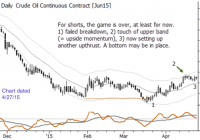
I initiated a short in crude oil back in July, and an astute reader sent me a good question. For many weeks/months, I had been operating with the assumption that crude oil was probably putting in a long-term bottom based on the action back in March/April of 2015; his question was how and why did I take a short against that bias. It’s a good and instructive question, so I thought I’d share the answer with you here. One of the advantages of writing about financial markets and publishing that work every day is that I have a record of what I was thinking and saying at any point in time. As I’ve written many times, I think journaling is one of the key skills of professional trading – this is a form of that. Let me set the background with some charts from a few months ago. A good place to start is in the aftermath of the 2014-2015 sell-off in crude oil. The market bounced in February 2015, set up another short attempt that more or less ran out of steam around the previous lows, and then rallied strongly off those March lows. In early April, I began to work with the idea that crude may have just put in a bottom. A chart says it better: (click to enlarge) Back in April, the case for a bottom in crude oil. Over the next few months, this thesis appeared to be playing out, but it’s important to remember that a bottom is a process. We don’t (usually) identify the absolute extreme of a move and then expect the market never to return. No, it’s far more likely that the market will go flat a while (check), and perhaps even re-test the previous extreme. This is normal, and it may even be those retests that really hammer the bottom in place. It’s easy to imagine hordes of traders thinking that crude oil is going to $20, entering short on a breakdown, and then watching in dismay as the market explodes to new highs after barely taking out the previous lows. A market will do whatever it can, at any time, to hurt the largest number of traders This, in fact, is nearly a principle of market behavior: A market will do whatever it can, at any time, to hurt the largest number of traders. That’s not just cynicism, I think it’s a legitimate consequence of the true nature of the market . Now, we certainly don’t want to be one of those gullible traders who gets tricked into shorting at exactly the wrong time, do we? So what do we do when the market gives us a nice, fat pitch right over the center of the plate, like this? A nice setup for a short, but what about the higher time frame conflict? And just to complete (or, perhaps, to further complicate) the picture, here’s the weekly chart from the same day: Thoughts on that higher time frame. So, just to clarify the situation here, in some bullet points, are the most important elements of market structure at the time we might have been thinking about a short entry: Within the past year, this market had a historic decline. Many people are inclined to think “Too far, too fast,” and that the move will reverse. On the other hand, maybe something fundamentally has changed. At the very least, we need to be aware that these might not be “normal” market conditions. After that historic decline, oil put in what looked like the first part of a bottom: A retest of lows, strong upside momentum off those lows, and then, daily consolidation patterns breaking to the upside. Following that step, the market went flat and dull, perhaps setting up a breakout trade. That breakout was to the downside, and a clear daily bear flag formed after the breakdown. Taking a short could mean going against the longer-term bottom (if it is forming), so what do we do? Many traders end up paralyzed with multiple time frames, as it’s easy to get overwhelmed with information. This is obviously a mistake, but there are also gurus who oversimplify the subject, saying, for instance, to only take a trade when it lines up with the higher-time frame trend. Though this idea is elegant and appealing, it falls short on several counts. For one, the best trades often come at turns, and if you wait to see an established trend, you’ll miss those trades; and even more importantly, the moving average-based trend indicators people use do not work like they think. (In fact, when a moving average trend indicator tells you a market is in an uptrend, at least for stocks, the stock is more likely go down !) Managing the conflicts How do we resolve all of this? I think this is a question that every trader must answer as part of his or her own trading plan. The one thing you probably cannot do is take each case as a new thing and try to make up rules for each situation. It’s far better to have a plan, and to then to follow that plan with discipline. For me, the answer is that a trade is just a trade. I have never been able to prove that having multiple time frames aligned actually increases the probability of those trades. (Though, those examples do sell books!) The way I think about it, if I have a higher-time frame trade that points up and a lower-time frame trade that points down, one of those trades will likely fail. I don’t know which, and I can’t know which in advance. If I knew the higher-time frame trend was more likely to work, I’d just trade that one, but in all intellectual honesty, I don’t know that. No one does. It’s possible that higher-time frame trend will fail because of the meltdown on the lower time frame, and if I’m positioned with that lower time frame, then I will be happy. It’s also possible I will get my first profit target even if the higher-time frame pattern “wins”, so I may be able to make money on both sides of the trade. Perhaps I want to skip the lower-time frame trade and just look for a higher-time frame trade around the previous low – that’s also a viable strategy. What matters is that I know what I will do in advance, and that I am honest about the limitations and constraints. We can only work within the laws of probability, and there are certainly limits to what can be known. It’s not a question of my competence as a trader, but of molding the methodology to fit the realities of the market. A trade is just a trade – avoid complications, and simplify.

Enhance Your Utility Sector Returns

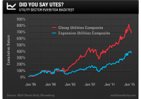
By Alan Gula Imagine you’re a pilot who is preparing to land an airplane. You’ve just eased up on the throttle, thereby slowing your airspeed. To compensate, you gently pull back on the yoke to increase the plane’s angle of attack. A buzzer suddenly goes off… it’s the stall warning. Your approach is too slow! The aircraft is at risk of rapidly losing altitude and the consequences could be dire. The concept of a stall speed can apply to economics, as well. That is, economic output tends to transition to a slow-growth phase (stall) at the end of an expansion before the economy falls into a recession. Right now, a buzzer should be sounding at the Federal Reserve because the U.S. economy has officially slowed below stall speed. Excluding the impact of inventories, real economic growth in the first half of 2015 was just 0.54%. Lackluster wage growth also indicates continued labor market slack. In the second quarter, the Employment Cost Index, a broad measure of labor costs, posted the smallest gain since records began in 1982. Indeed, recent data further support my view that the risk of a meaningful rise in interest rates is low. And because we’re in a subdued economic growth and inflation environment, I believe that the utilities – electricity, gas, and water companies – continue to be viable investments. However, we must be wary of valuations, especially for relatively high-yielding securities. Investors starved for yield have bid up prices across the utility sector, pushing average valuations to historically high levels. We also want to avoid utilities that are excessively levered. Luckily, we can help alleviate both of these concerns with the trusty enterprise value-to-EBITDA (EV/EBITDA) ratio. Remember, the EV/EBITDA ratio compares the total stakeholder value net of cash with the total cash flows available to all stakeholders. Firms with high equity valuations and/or high debt levels have higher (less attractive) EV/EBITDA ratios. To illustrate the power of this valuation metric, I ran a backtest starting in June 1995. Here, my universe of stocks is U.S.-listed utilities with market caps above $1 billion. The stocks are ranked based on EV/EBITDA, and the top two deciles (cheapest 20%) are included in the Cheap Utilities Composite. The bottom two deciles (most expensive 20%) are included in the Expensive Utilities Composite. The screen is rerun each month and the composites change as the companies’ valuations change. The constituents are allocated to on an equal-weight basis and the cumulative total return (dividends reinvested) for each composite is tallied. The results of this backtest are shown below: As you can see, the Expensive Utilities Composite produces a cumulative return of 363% over 20 years. Meanwhile, the Cheap Utilities Composite gained an incredible 680%, which actually trounces the 451% total return posted by the mighty S&P 500 over this same time frame. Clearly, there’s an edge to buying cheap utilities based on the EV/EBITDA ratio. Furthermore, the cheap utilities also experienced smaller declines. The largest drawdown (peak to trough decline) that you would’ve experienced in the Expensive Utilities Composite was 40%, compared with just 35% for the Cheap Utilities Composite. Higher returns with lower volatility – the best of both worlds. Currently, the median EV/EBITDA for all U.S.-listed utilities with market caps greater than $1 billion is 9.9, which is relatively high. The current constituents of the Cheap Utilities Composite, which includes companies such as AES (NYSE: AES ), Ameren (NYSE: AEE ), AGL Resources (NYSE: GAS ), and Pinnacle West (NYSE: PNW ), have a median EV/EBITDA of 7.8. To make sure that the utilities you own are trading at reasonable valuations, the Key Statistics page on Yahoo! Finance has EV/EBITDA along with a host of other data. In the midst of persistently low interest rates and with an economy below stall speed, utilities are attractive investments that can help protect your portfolio from broader stock market declines. Just make sure your utilities are cheap with a low degree of leverage. Original Post