Tag Archives: load

Adding The Agriculture ETF And A Portfolio Update

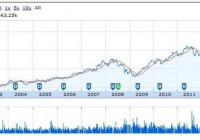
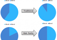
One of our holdings, (Nestle) may have lower profits in the short term due to the strength of the Swiss Franc. Nevertheless we are holding this stock long term. Our long bond position is performing very well. It gives our portfolio stability and it acts as a hedge against falling prices in our equities. We have added 2 new agricultural ETFs to our portfolio. We are investing with the trend for the time being but I expect to deploy more capital into DBA soon. First of all, an update on our 1% portfolio. In our equity asset class, we are holding Nestle ( OTCPK:NSRGY ). As many of you know, the Swiss National Bank announced the abandonment of the currency peg with the euro. The following day a follower emailed me and asked if we were going to continue to hold Nestle as this company is headquartered in Switzerland. The answer is a definite yes! We may have some downward movement in Nestle in the short term as the Swiss Franc strengthens against other currencies. Nestle sells all over the world in other currencies and if these international currencies weaken substantially against the Swiss Franc, then Nestle profit margins may be hit as their accounts are filed in Swiss Francs. Nevertheless this is a currency issue, not a fundamental issue. The stock has excellent fundamentals and has been in strong bull mode since 2001 (see chart). The company is yielding just under 3% and has increased its dividend for the past 18 years straight! Similar to American Express (NYSE: AXP ), we are going to stay the course with this holding. (click to enlarge) Our bond position in the Vanguard Total Bond Market ETF (NYSEARCA: BND ) is creating a lot of controversy as many think our stake in this asset class is too large. Currently we have $100k invested in this asset class. Let me explain the reasoning behind this decision. I learned early on in my investing career that if your money is divided equally but your investments are not equal in their risk, you are not balanced. Most portfolios are made up of stocks and the problem with these types of portfolios is that they don’t protect you in bear markets. Today (27-1-2015) we have the S&P falling sharply and bonds rallying. This has been the case more or less since the 2008 equity crash. U.S. Bonds have been a flight to safety when U.S. equities have fallen. A portfolio is not just made up of asset classes in equal proportions. We must also understand how these asset classes compare to each other. In the short term, our bond position is going to act as a hedge against our stock positions and we will also collect the 2% yield it pays out. We need to have a portfolio that will make us money if we have inflation or deflation or if we have economic growth or recessions. Every asset class has its bull markets and bear markets and nobody (no matter who they are) can predict the future. We have had the real estate bull market in the early 2000’s and then the stock market revival since 2008. What asset class will provide the next bull run? Gold, Agriculture, will real estate come back strong? The fact of the matter is that nobody knows and until new trends start to take place, we will stay long our bond position Finally, we are going to add an agricultural presence to our portfolio. These ETFs are going to give our portfolio stability as they are not volatile. I compared the Market Vectors Agribusiness ETF (NYSEARCA: MOO ) and the PowerShares DB Agriculture ETF (NYSEARCA: DBA ) (see chart below): (click to enlarge) We will invest an initial $70k into this sector with $50k going into the Market Vectors Agribusiness ETF and $20k into the PowerShares DB Agriculture ETF. The Market Vectors Agribusiness ETF has vastly outperformed The PowerShares DB Agriculture Fund over the last 7 years because it’s a fund invested in U.S. companies in this sector. Moreover, it definitely has been helped by the stock market rally since 2008. However, I expect the trend in the above chart to change in the near future. When it does, we will rebalance this sector and invest more heavily into DBA. This fund solely concentrates on price movement of the agricultural commodities (corn, sugar, wheat, etc.) and that is where I think the big gains will be in this sector going forward. Editor’s Note: This article discusses one or more securities that do not trade on a major exchange. Please be aware of the risks associated with these stocks. Now that you’ve read this, are you Bullish or Bearish on ? Bullish Bearish Sentiment on ( ) Thanks for sharing your thoughts. Why are you ? Submit & View Results Skip to results » Share this article with a colleague

Does ‘Sharpe Parity’ Work Better Than ‘Risk Parity?’

By Wesley R. Gray Strategies employing Risk Parity have been favored by mutual funds and other market participants the past few years. The attraction of risk parity strategies is the great story associated with the approach and the historical performance over the past 30 years has been favorable. However, there is an argument that historical risk parity performance has been driven by leveraged exposure to Treasury Bonds, which have been on an epic tear the past ~30 years. Nonetheless, good stories such as risk parity never die on Wall Street, they merely adapt and overcome. This white paper by UBS highlights skepticism around risk parity and presents a different, but related asset allocation method: Sharpe Parity. Risk Parity Background: As you may recall, risk parity identifies weights that equalize “risk” across asset classes. Let’s first review a simple risk parity example. Here is a visual interpretation of how risk parity works. If we allocate to a 60/40 stock/bond portfolio on a dollar-weighted basis, on a risk-contribution basis, we might be getting 90% of our risk from stocks and 10% of our risk from bonds. Risk parity comes to the so-called rescue. Risk parity suggests that we rejigger the dollar-weighted 60/40 portfolio in such a way that the risk contributions end up being 50% driven by bond exposure and 50% driven by stock exposure. In other words, our “risk contributions” are at parity, hence the title “risk parity.” How does this work in practice using the most basic version of risk parity outlined in the Asness, Frazzini, and Pedersen paper: (click to enlarge) Source: Leverage Aversion and Risk Parity (2012), Financial Analysts Journal, 68(1), 47-59 But UBS Doesn’t like Risk Parity. Why? As per their own research: Risk Parity ignores return and focuses only on risk; Risk Parity uses volatility as the sole measure of risk, while neglecting other credit-related risks, such as default risk and illiquidity; Risk Parity encounters huge drawdowns if bonds and equity sell off together; A low nominal return world makes recovery from risk parity drawdowns difficult. UBS proposes a new asset allocation strategy, which shares some concepts with risk parity, but in their approach risk parity’s “standard deviation” is replaced with an estimate for an asset’s Sharpe Ratio. Here’s an explanation of the concept: “Think about it this way: if asset X has a Sharpe ratio of 2 it means that we have two units of return for 1 unit of risk, while asset Y with a Sharpe ratio of 1 gives us only 1 unit of return for the same amount of risk. In that case we construct a portfolio with the weight for asset X being double the weight of asset Y.” Strategy Background: This approach makes some sense, as it seems to account for return as well as risk. This approach is also in line with modern portfolio concepts such as mean-variance analysis, where investors want to maximize marginal Sharpe Ratios to create the so-called “tangency portfolio” that all MBA 101 students know and love. But how does “Sharpe Parity” stand up to empirical scrutiny? In order to address this question, we compare 4 asset allocation approaches: Equal-weight allocation , an equal-weight allocation with a Simple Moving Average rule , simple Risk Parity , and Sharpe Ratio Parity . Equal-weight (EW_Index): monthly rebalanced equal-weight portfolios. Simple Moving Average (EW_Index_MA): calculate a simple moving average each month (12 month average); if the MA rule is triggered (when the current price > 12 month moving average), buy risk, or else, allocate to the risk-free asset. Risk Parity: follow the simple risk parity algorithm; use a look-back period of 36 months for the “standard” risk parity model. Sharpe Parity: use a look-back period of 36 months for the Sharpe Parity model; if an asset has a negative Sharpe Ratio, this asset’s weight will be 0; note that if all the assets’ Sharpe Ratios are negative, the strategy will allocate 100% to the risk-free asset. Data Description: To test these 4 strategies, we apply them to the “IVY 5” asset classes: SP500 = SP500 Total Return Index EAFE = MSCI EAFE Total Return Index REIT = FTSE NAREIT All Equity REITS Total Return Index GSCI = GSCI Index LTR = Merrill Lynch 7-10 year Government Bond Index (click to enlarge) The “IVY 5” Concept. Click to enlarge. Our simulated historical performance period is from 1/1/1980 to 7/31/2014. Results are gross, and thus do not include the effects of fees. All returns are total returns and include the reinvestment of distributions (e.g., dividends). Data was obtained via Bloomberg. Indexes are unmanaged, do not reflect management or trading fees, and one cannot invest directly in an index. Please see the disclosures at the end of this document for additional information. Sharpe Parity has a slightly higher CAGR. However on a risk-adjusted basis, Equal Weight MA and Risk Parity outperform the Sharpe Parity system, as reflected in their higher sharpe and sortino ratios. The simple moving average technique has the lowest drawdown and the best overall risk-adjusted performance. (click to enlarge) The results are hypothetical results and are NOT an indicator of future results and do NOT represent returns that any investor actually attained. Please see disclosures for additional information. Additional information regarding the construction of these results is available upon request. Does Lookback period matter? Next, we change the look-back period from 36 months to 3 months, which is identical to the lookback period used in the UBS whitepaper. Here’s the result: Sharpe Parity based on a 3 months lookback period has larger CAGR, but also has larger drawdowns, on a monthly, worst case, and cumulative basis. Sharpe and sortino ratios are worse than the 36 month lookback version. (click to enlarge) The results are hypothetical results and are NOT an indicator of future results and do NOT represent returns that any investor actually attained. Please see disclosures for additional information. Additional information regarding the construction of these results is available upon request. Conclusions Based on these results, it seems hard to conclude that Sharpe Parity, particularly with a 3 month look-back period, offers a clear-cut advantage over traditional Risk Parity approaches. In fact, on a risk-adjusted basis, it compares poorly. Based on this analysis, it would appear that simple equal-weight portfolios with trend-following rules have worked better than more complicated risk parity or sharpe parity systems. Original Post

Tech ETF IBB Brings Plenty Of Risk But It Fits Nicely In A Portfolio

Summary IBB has a respectably low correlation to SPY, but the ETF is quite volatile on its own. The ETF doesn’t make sense for investors that are retiring, but it works fine for investors not seeking yield. I’d rather see lower expense ratios, but they aren’t bad enough to make the ETF unattractive. I’ll share my findings on ideal exposure levels. Investors should be seeking to improve their risk adjusted returns. I’m a big fan of using ETFs to achieve the risk adjusted returns relative to the portfolios that a normal investor can generate for themselves after trading costs. I’m working on building a new portfolio and I’m going to be analyzing several of the ETFs that I am considering for my personal portfolio. A substantial portion of my analysis will use modern portfolio theory, so my goal is to find ways to minimize costs while achieving diversification to reduce my risk level. In this article I’m reviewing the iShares Nasdaq Biotechnology ETF (NASDAQ: IBB ). What does IBB do? IBB attempts to track the investment results of an index composed of pharmaceutical and biotechnology equities. The ETF falls under the category of “Health”. Does IBB provide diversification benefits to a portfolio? Each investor may hold a different portfolio, but I use (NYSEARCA: SPY ) as the basis for my analysis. I believe SPY, or another large cap U.S. fund with similar properties, represents the reasonable first step for many investors designing an ETF portfolio. Therefore, I start my diversification analysis by seeing how it works with SPY. I start with an ANOVA table: (click to enlarge) The correlation is about 69%, which is low enough that I’m expecting to see significant diversification benefits. Standard deviation of daily returns (dividend adjusted, measured since January 2012) The standard deviation isn’t going to make a strong case for investing in IBB. For the period I’ve chosen, the standard deviation of daily returns was 1.391 %. For SPY, it was 0.736% over the same period. Clearly, SPY appears to be the safer of the two investments. Mixing it with SPY I also run comparison on the standard deviation of daily returns for the portfolio assuming that the portfolio is combined with the S&P 500. For research, I assume daily rebalancing because it dramatically simplifies the math. With a 50/50 weighting in a portfolio holding only SPY and IBB, the standard deviation of daily returns across the entire portfolio is 0.987%. The risk level on the portfolio drops relative to only holding SPY because of the diversification benefits that come from the 69% correlation. If the position in SPY is raised to 80% while IBB is used at 20% the standard deviation of daily returns drops down to 0.807%. In practice, I think the best way to use IBB is a position smaller than 20% and used in a diversified portfolio. The low correlation makes a very strong case for using IBB in a small position to enhance diversification. I would lean to limiting exposure to around 5%. At 5%, the standard deviation of the portfolio would have been 0.749%. Compared to SPY at .736%, this is a fairly low increase in the risk level measured by the standard deviation. Most of the additional deviation introduced by IBB has been effectively diversified away once the position hits 5% in a portfolio that is primarily SPY. Why I use standard deviation of daily returns I don’t believe historical returns have predictive power for future returns, but I do believe historical values for standard deviations of returns relative to other ETFs have some predictive power on future risks and correlations. Yield & Taxes The distribution yield is .15%. Simply put, the ETF doesn’t make much sense for a retiring investor that wants to use portfolio yields as a large part of their retirement income. Sure, they could sell shares to generate income, but that may create a temptation to change the portfolio strategy at the wrong time. Expense Ratio The ETF is posting .48% for an expense ratio, which is higher than I’d like to see. Unfortunately, most ETFs have expense ratios higher than I’d like to see. This isn’t bad compared to other ETFs, though it is substantially higher than SPY at .09%. Market to NAV The ETF is trading at a .01% premium to NAV currently. I think any ETF is significantly less attractive when it trades above NAV. A .01% premium is not enough to matter though. Investors should check prior to placing an order, but the liquidity in IBB should be a great hedge against any meaningful premiums or discounts. Largest Holdings The diversification within the ETF is pretty weak. For a very long term holder it might make sense to replicate the ETF by just buying the underlying securities and taking higher trading costs to eliminate the expense ratio. (click to enlarge) Investing in the ETF is largely relying on modern portfolio theory. The argument for the investment is the respectably low correlation of the portfolio to the major U.S. index funds. Making an investment requires a belief that markets are at least somewhat efficient so that the companies within the portfolio will be reasonably priced. Conclusion The trading volume for the ETF is fairly solid. Recently the average volume was about 1.7 million shares per day. During my three year sample period there were 0 days in which no shares were trading hands. Based on that solid liquidity, I think the statistics are fairly reliable and find the ETF appealing under modern portfolio theory if investors have a large enough portfolio have less than 5% invested in IBB and still have the position be meaningful. Due to the small percentage of the portfolio that I would suggest for such a volatile portfolio, it makes more sense for investors that have access to some free trading on IBB or investors that have a portfolio large enough that the trading costs are inconsequential. The ETF has been on a tear over the last 3 years. During the period the ETF is up about 190%, but since it still trades at NAV that is simply reflecting the incredible growth of the underlying companies. Investors doing some quick research may see that the Beta of the ETF is .83. That value depends on measuring the ETF relative to a benchmark associated with the index rather than comparing the risk level to SPY.