Tag Archives: latest-articles

Value Investing: Have You Been Using The Wrong Quality Ratio?

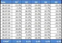
By Tim du Toit Do you think adding a company quality ratio to your investment strategy can make a difference to your returns? As you know we are skeptical, as our experience testing quality ratios in the research paper Quantitative Value Investing in Europe: What Works for Achieving Alpha was mixed. What doesn’t work We found that Return on invested capital (ROIC) and return on assets (ROA) weren’t good predictors of returns. Even though high-quality companies did do better than low-quality companies (low ROIC and ROA) returns did not increase in a linear way as you moved from low-quality to high-quality companies. And if you only invested in high-quality companies, it would not have helped you to consistently beat the market. A better quality ratio? Our thinking on quality ratios changed when we read a very interesting research paper called The Other Side of Value: The Gross Profitability Premium by Professor Robert Novy-Marx in which he defined a company quality ratio performed as well as a valuation ratio. How calculated Professor Novy-Marx defined a quality company as one that had a high gross income ratio (let’s call it Quality Novy-Marx ), which he calculated by dividing gross profits by total assets . He defined gross profit as sales minus cost of sales and assets simply total assets as shown in the company’s balance sheet (current assets + fixed assets). Does it work? In the paper Professor Novy-Marx shows that this simple ratio has about the same predictive return value as the price to book ratio in spite of companies with a high gross income ratio (Quality Novy-Marx) being a lot different if you compare them to undervalued companies with a low price to book ratio. Companies with a high Quality Novy-Marx ratio generated significantly higher average returns than less profitable companies in spite of them, on average, having a higher price to book ratio (more expensive) and higher market values. Because value (low price to book) and profitability (high Quality Novy-Marx ratio) strategies’ returns are negatively correlated (the one goes up when the other goes down), the two strategies work very well together. So much so that Professor Novy-Marx in the paper suggests that value investors can capture the full high-quality outperformance without taking on any additional risk by adding a high quality strategy to an existing value strategy. If you do this he found that this reduces overall portfolio volatility, in spite of it doubling your exposure to the stock market. We also tested it We of course also wanted to test if the Quality Novy-Marx ratio works on the European stock markets. Our back test (on European companies) over just less than 12 years from July 2001 to March 2013 came up with the following result: Source: Quant-Investing.com 1 Quintiles 2 Compound Annual Growth Rate ( OTCPK:CAGR ) As you can see the results are (apart from Q1 to Q2) linear, which means as you move from low-quality companies (Q5) to high-quality companies (Q1) returns increase every time. Also high quality companies (Q1) did substantially better than low-quality companies (Q5). This clearly shows that the Quality Novy-Marx ratio is a very good ratio to add to how you search for investment ideas. Substantially outperformed the market High-quality companies also substantially outperformed the index. The STOXX Europe 600 index over the same period had a compound annual growth rate of -0.82%, worse than even the worse quintile, most likely because of the banks being included in the index (not in the back test universe because you cannot calculate the Quality Novy-Marx ratio for them). In summary From these two back tests you can see that adding quality companies, defined as companies with high gross profits to total assets can definitely add to your investment returns. We have not tested it but Professor Novy-Marx mentions that if you are a value investor, quality companies have the ability to increase your returns and decrease the volatility of your portfolio. But if you add this quality ratio to your screens, you will find companies that are not undervalued, which is something that value investors will have to get used to. Where can you find it? In the screener you can select the gross income ratio (called Gross Margin (Marx)) as a ratio in one of the four sliders as shown below. Or you can select the Gross Margin (Marx) as a column in your screen which will allow you to filter and sort the Gross Margin (Marx) values.

Does ‘Sharpe Parity’ Work Better Than ‘Risk Parity?’

By Wesley R. Gray Strategies employing Risk Parity have been favored by mutual funds and other market participants the past few years. The attraction of risk parity strategies is the great story associated with the approach and the historical performance over the past 30 years has been favorable. However, there is an argument that historical risk parity performance has been driven by leveraged exposure to Treasury Bonds, which have been on an epic tear the past ~30 years. Nonetheless, good stories such as risk parity never die on Wall Street, they merely adapt and overcome. This white paper by UBS highlights skepticism around risk parity and presents a different, but related asset allocation method: Sharpe Parity. Risk Parity Background: As you may recall, risk parity identifies weights that equalize “risk” across asset classes. Let’s first review a simple risk parity example. Here is a visual interpretation of how risk parity works. If we allocate to a 60/40 stock/bond portfolio on a dollar-weighted basis, on a risk-contribution basis, we might be getting 90% of our risk from stocks and 10% of our risk from bonds. Risk parity comes to the so-called rescue. Risk parity suggests that we rejigger the dollar-weighted 60/40 portfolio in such a way that the risk contributions end up being 50% driven by bond exposure and 50% driven by stock exposure. In other words, our “risk contributions” are at parity, hence the title “risk parity.” How does this work in practice using the most basic version of risk parity outlined in the Asness, Frazzini, and Pedersen paper: (click to enlarge) Source: Leverage Aversion and Risk Parity (2012), Financial Analysts Journal, 68(1), 47-59 But UBS Doesn’t like Risk Parity. Why? As per their own research: Risk Parity ignores return and focuses only on risk; Risk Parity uses volatility as the sole measure of risk, while neglecting other credit-related risks, such as default risk and illiquidity; Risk Parity encounters huge drawdowns if bonds and equity sell off together; A low nominal return world makes recovery from risk parity drawdowns difficult. UBS proposes a new asset allocation strategy, which shares some concepts with risk parity, but in their approach risk parity’s “standard deviation” is replaced with an estimate for an asset’s Sharpe Ratio. Here’s an explanation of the concept: “Think about it this way: if asset X has a Sharpe ratio of 2 it means that we have two units of return for 1 unit of risk, while asset Y with a Sharpe ratio of 1 gives us only 1 unit of return for the same amount of risk. In that case we construct a portfolio with the weight for asset X being double the weight of asset Y.” Strategy Background: This approach makes some sense, as it seems to account for return as well as risk. This approach is also in line with modern portfolio concepts such as mean-variance analysis, where investors want to maximize marginal Sharpe Ratios to create the so-called “tangency portfolio” that all MBA 101 students know and love. But how does “Sharpe Parity” stand up to empirical scrutiny? In order to address this question, we compare 4 asset allocation approaches: Equal-weight allocation , an equal-weight allocation with a Simple Moving Average rule , simple Risk Parity , and Sharpe Ratio Parity . Equal-weight (EW_Index): monthly rebalanced equal-weight portfolios. Simple Moving Average (EW_Index_MA): calculate a simple moving average each month (12 month average); if the MA rule is triggered (when the current price > 12 month moving average), buy risk, or else, allocate to the risk-free asset. Risk Parity: follow the simple risk parity algorithm; use a look-back period of 36 months for the “standard” risk parity model. Sharpe Parity: use a look-back period of 36 months for the Sharpe Parity model; if an asset has a negative Sharpe Ratio, this asset’s weight will be 0; note that if all the assets’ Sharpe Ratios are negative, the strategy will allocate 100% to the risk-free asset. Data Description: To test these 4 strategies, we apply them to the “IVY 5” asset classes: SP500 = SP500 Total Return Index EAFE = MSCI EAFE Total Return Index REIT = FTSE NAREIT All Equity REITS Total Return Index GSCI = GSCI Index LTR = Merrill Lynch 7-10 year Government Bond Index (click to enlarge) The “IVY 5” Concept. Click to enlarge. Our simulated historical performance period is from 1/1/1980 to 7/31/2014. Results are gross, and thus do not include the effects of fees. All returns are total returns and include the reinvestment of distributions (e.g., dividends). Data was obtained via Bloomberg. Indexes are unmanaged, do not reflect management or trading fees, and one cannot invest directly in an index. Please see the disclosures at the end of this document for additional information. Sharpe Parity has a slightly higher CAGR. However on a risk-adjusted basis, Equal Weight MA and Risk Parity outperform the Sharpe Parity system, as reflected in their higher sharpe and sortino ratios. The simple moving average technique has the lowest drawdown and the best overall risk-adjusted performance. (click to enlarge) The results are hypothetical results and are NOT an indicator of future results and do NOT represent returns that any investor actually attained. Please see disclosures for additional information. Additional information regarding the construction of these results is available upon request. Does Lookback period matter? Next, we change the look-back period from 36 months to 3 months, which is identical to the lookback period used in the UBS whitepaper. Here’s the result: Sharpe Parity based on a 3 months lookback period has larger CAGR, but also has larger drawdowns, on a monthly, worst case, and cumulative basis. Sharpe and sortino ratios are worse than the 36 month lookback version. (click to enlarge) The results are hypothetical results and are NOT an indicator of future results and do NOT represent returns that any investor actually attained. Please see disclosures for additional information. Additional information regarding the construction of these results is available upon request. Conclusions Based on these results, it seems hard to conclude that Sharpe Parity, particularly with a 3 month look-back period, offers a clear-cut advantage over traditional Risk Parity approaches. In fact, on a risk-adjusted basis, it compares poorly. Based on this analysis, it would appear that simple equal-weight portfolios with trend-following rules have worked better than more complicated risk parity or sharpe parity systems. Original Post

Are Multi-Asset Funds A Threat To The Fund Industry?

By Detlef Glow The chase for yield by all kinds of investors has driven up the popularity of so-called multi-asset funds, since the funds promise to be widely diversified and therefore able to generate returns from all kinds of assets. In a number of cases the promise also extends to all kinds of market conditions, since some of the funds have the ability to use shorts or so-called market-neutral strategies. With regard to the investment objectives of multi-asset funds, these funds can be considered as really actively managed funds. That mixed- or multi-asset funds are privileged products for European investors is shown in the impressive inflows these funds have been able to gather. Asset allocation funds were not only the best selling fund sector for 2013 (+€61.6 bn), they also led the table for the first 11 months of 2014. In this period asset allocation products gathered €63.3 bn, far ahead of the second and third best selling sectors: mixed-asset conservative (+€27.9 bn) and bonds EUR (+€27.5 bn). The strong inflows into the multi-asset sector, combined with the fact that more and more fund promoters are launching multi-asset products to benefit from this trend, have raised questions and concerns about multi-asset products. One of these questions is whether all of these new managers are able to handle multi-asset portfolios, especially in tough times. Will these managers be able to meet the expectations of their investors in bear markets? The fear behind this question is linked to the negative image of the fund industry that stemmed from a number of absolute return funds failing to meet their goals during the 2008 financial crisis. From my point of view this is a valid concern: some managers may not be able to handle rough markets. They might not be experienced in the use of shorts, or they may not have the right risk management tools in place. Another point of concern is that some asset managers try to run their multi-asset portfolios with small teams to cover a large number of asset classes, or they are managing these portfolios in addition to other portfolio management tasks. In this regard, investors should make sure the fund management team of their fund is focused on the multi-asset portfolio and has enough resources to handle all the asset classes in the portfolio. The second major concern I have heard often in recent months is about fund flows. Since multi-asset products seem to have been the investment of choice of both institutional/professional and private investors in the past two years, some observers state that the flows might have reached their peak. Investors may start to pull out their money from these funds, which could lead to major outflows and therefore disruptions in some asset classes. I do not think that private investors will stop investing in multi-asset products as long as the funds fulfill their investment objectives and the goals of the investors. But it looks a bit different on the institutional side. New regulations such as Solvency II, with its high reporting standards, may cause some outflows from mutual funds, regardless of whether the fund promoters are able to deliver holdings data and other statistics on time. Another reason for outflows might be because asset managers are using multi-asset funds instead of buying the single building blocks and building multi-asset portfolios of their own. That would be the only way for them to have their asset allocation fully under control. From my point of view both concerns are valid; institutional outflows could easily offset inflows, which might cause outflows from the asset allocation sector. Even so, I would not expect any major disruptions in the utilized asset classes from this, since major outflows are unlikely to happen from one day to the next. In addition, I don’t think all the institutional investors who have bought multi-asset funds are able to manage this kind of portfolio in-house and therefore need an external manager to participate in these broadly diversified investment strategies. I would assume some questions and concerns around multi-asset funds are valid, but as long as at least the major funds in this market segment continue to deliver on their investment objective, the fund category is not a major threat for the European mutual fund industry. From my point of view, the major risk for the fund industry would be if one of the top-selling funds in this segment fails to deliver on its investment objective or faces major losses during a crisis. That would once again damage the reputation of the fund industry, which might then irrevocably lose investors’ trust. The views expressed are the views of the author, not necessarily those of Thomson Reuters.