Tag Archives: alt-investing

The Beginner’s Guide To Volatility: ZIV

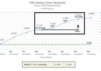
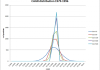
Summary We will cover the basics of ZIV. Examples of trading strategies for the mid-term futures. Current advice on ZIV. Welcome to the final part of The Beginners Guide to Volatility. I highly encourage you to view the two articles below, unless you have already read them. Some terms in this article were previously explained in the first two parts. Part One: The Beginner’s Guide To Volatility: VXX Part Two: The Beginner’s Guide To Volatility: XIV VelocityShares Daily Inverse VIX Medium-Term ETN (NASDAQ: ZIV ) This article will focus on the mid-term VIX futures. To be clear, these products are not the same as the short-term futures products we have discussed before. Some things are similar and others are very different. As a basis for discussion, we will use the inverse product ZIV. I really don’t recommend any other mid-term futures products. What are the mid-term futures? How would an inverse fund operate in the mid-term futures? See below: (click to enlarge) The mid-term futures span months four through seven. An inverse fund, which means in reverse order, sells short month seven’s contract. The fund will hold that contract (short) until selling it when it reaches month four. This process typically takes about 90 days depending on the month and expiration date of the VIX futures. As you may recall from the previous two articles, VIX futures are not the VIX Index and they trade independently of the market and level of stock prices. If you are on vixcentral.com, below the individual months you will see the month seven to four contango box. I have edited this into the above graphic. The first box represents the total percentage of contango or backwardation from month seven to four. For more on these terms, please view the first two articles in this series. The second box represents the estimated amount of contango or backwardation you could expect to profit/loss from during the next 30 days. It takes the first box and divides it by three. Again this is just an estimate. Contango/Backwardation in Mid-Term Futures Charts above and below made by Nathan Buehler using data from The Intelligent Investor Blog . Below, you will see an overlay of ZIV using the same time values to give you a clearer view of the data: Context It is important to view the above chart to put the mid-term futures into context. Although the data is back-tested, it is still relevant and useful. Had you viewed the current data alone (see below), it would appear mid-term future rarely go into backwardation. For the most part, this is true; however, you should be aware of negative economic events that would cause a deeper and more prolonged trek through backwardation. (click to enlarge) Why Consider Inverse Mid-Term Futures? Inverse mid-term futures provide a less volatile bet on decreasing volatility and/or sideways to rising markets. The best reward for your risk would be investing in these products after a dramatic and prolonged spike in the mid-term VIX futures. Historically, investing in mid-term futures now would give you a high risk and minimum reward scenario. See below for an example of a winning strategy: Winning Strategy: Let’s review two strategies that would work well. Buy ZIV once futures re-enter contango from backwardation. Risk of backwardation reappearing. Wait for backwardation and buy ZIV once 5% contango is reached. Visual (click to enlarge) Let’s go over the positives, negatives, and key takeaways with this strategy. Positives: Mid-term futures are already less volatile and less risky than short-term futures. This strategy, especially strategy two, is conservative in managing risk. Negatives: With strategy one, futures could reenter backwardation causing large losses. This opportunity will only occur once a year on average. Some periods may go longer without seeing backwardation present in the mid-term futures. It has been almost four years since the mid-term futures were in backwardation. Takeaways: Your focus on this decision should be in the strength of the U.S. economy and the ever more important global economic impact on the U.S. You need a positive economic outlook and improving or stable economic conditions for this to work as intended. Liquidity One thing you will notice about ZIV in comparison to short-term futures products is the drastically lower volumes. Average volume over the past three months is about 62,000, representing around $2.5-$3 million in transactions per day. As of writing, the fund has $123 million in assets under management (AUM). This represents about 2% of the fund being traded per day. When compared with the ProShares Ultra VIX Short-Term Futures ETF (NYSEARCA: UVXY ) that fund had about $342 million in AUM, and with its near-term average volume of 12 million shares, that represents around $360 million or over 100% of the assets in the fund being traded per day. ZIV will attract investors that are not looking for a day trade and have more of a buy-and-hold or longer-term view of the market. The low volume does not make this an illiquid investment. Conclusion The inverse mid-term VIX futures offer you another way to invest in volatility. It is a much slower pace than the short-term futures but also carries a more moderate level of risk if backwardation persists for a long period of time. Should things turn south, this product is much more forgiving in allowing you to exit a position. Short-term products often react much worse to immediate events. Now is not an opportune time to invest in the mid-term futures, but this article should have given you a good indication of what conditions would look like when the opportunity arises. I appreciate you reading this series, and I hope it continues to serves as a foundational education piece for volatility investors for years to come. My best advice is to fully educate yourself before investing in any VIX-related products. Knowledge is power and very important with this asset class. Disclosure: I/we have no positions in any stocks mentioned, and no plans to initiate any positions within the next 72 hours. (More…) I wrote this article myself, and it expresses my own opinions. I am not receiving compensation for it (other than from Seeking Alpha). I have no business relationship with any company whose stock is mentioned in this article.

The Low Volatility Anomaly: Overconfidence Bias

This series offers an expansive look at the Low Volatility Anomaly, or why lower risk stocks have historically produced stronger risk-adjusted returns than higher risk stocks or the broader market. This article hypothesizes that cognitive biases like the overconfidence bias contribute to the Low Volatility Anomaly. Like previous pieces in this series, this article covers a deviation between model and market that may contribute to the outperformance of low volatility strategies. A cognitive bias is a deviation in judgment where people draw inferences in an illogical fashion. As discussed in the last piece in this ongoing series on lottery preferences , cognitive biases can impact investment decision-making and likely contribute to the Low Volatility Anomaly. This article will discuss an additional cognitive biases that could contribute to this phenomenon – the overconfidence bias. The overconfidence bias suggests that a person’s subjective confidence in their own judgment is reliability greater than the objective accuracy of those judgments. The most oft cited example of the overconfidence bias is the 1980 finding by Ola Svensson that ninety-three percent of American drivers rate themselves better than the median. Traveling back from the highway to the Capital Asset Pricing Model (CAPM) assumptions, the model calls for homogeneous investor expectations, including expected values, standard deviations, and correlation coefficients. Valuing investments necessarily involves forecasting as a means to assessing tradeoffs between risk and return. Empirical evidence suggests that most people form confidence intervals that are too narrow. Borrowing from studies by Fischoff, Slovic, and Lichtenstein (1977) and Alpert and Raiffa (1982) , I conducted a similar study during a lecture to a fixed income class at my undergraduate alma mater in the fall of 2014. The students were asked a set of ten questions with numeric answers and asked to bound their answer by a confidence interval such that there was a ninety percent chance that their numeric answer would fall within the range. The ten questions were as follows: What is the population of the state? What is the seating capacity of the football stadium? What is number of different undergraduate majors at the University? What were the revenues of the athletic program in the previous year? What was the number of degrees conferred in the most recent academic year? What is the current yield level of the 30-year Treasury? What is the size of the U.S. Gross Domestic Product? What was the total number of jobs created in the U.S. in 2014? What was the total number of automobiles sold in the U.S? What is the U.S. Median Household Income? At a ninety percent confidence interval, half the class should have had nine or more results inside their confidence interval. Of the roughly thirty-five students, none had nine. Or eight. Or seven. Or six. Two students had five of their answers inside their bounds, but most of the students had between two and four. The class was overconfident. The first five questions were on the world around them at college, and the second five questions were on basic economic statistics. These topics should have yielded far better forecasts than the multi-year prognostications of market or security variables inherent in investment selection. The students did poorly – as poorly as the author when he first completed a similar exercise. The point of the exercise (aside from breaking up the monotony of my lecture) was to illustrate the overconfidence bias to the class. Overconfidence can drastically damage investment returns. Given the geographic proximity of the university to some of the nation’s leading onshore oil and gas resources, the rapid and unexpected drawdown in oil prices at the time of the lecture and the related implications on energy-related assets proved salient to the audience. Additional examples of the overconfidence bias given in the lecture included persistent overestimates of economic growth from the International Monetary Fund and Federal Reserve post-crisis, and the poor job of private and public sector economists at forecasting long-term interest rates, which were at the time rallying sharply in the face of consensus estimates for rising rates. Like the students surveyed, professional investors have proved similarly overconfident. Active managers implicitly assume that they are capable of beating their benchmark despite long-run evidence demonstrating that the average active manager fails to accomplish this feat on average over time ( Fama, French 2009 ). The collective overconfidence by the cadre of active managers violates that CAPM assumption of rationality and could be a factor that contributes to the Low Volatility Anomaly. If a manager is truly as skilled as they believe, then participation in higher volatility segments of the market offer the largest return proposition to capitalize on their perceived skill. If that same manager believed that the market was likely to fall, then they would not choose to invest in low volatility assets, which would outperform on a relative basis, but choose to exit the market entirely to outperform on an absolute basis. This overconfidence bias then likely contributes to the outperformance of low volatility stocks (referenced by SPLV ) relative to high beta stocks (referenced by SPHB ) depicted in the introductory article to this series . Further connecting the overconfidence bias to investment returns, we see more activity from market optimists than pessimists. Perhaps married to the market frictions inherent in the Leverage Aversion Hypothesis , the market in general is far less likely to short high volatility assets than it is to buy them. With skeptics more often sidelined than short, high beta assets with a more diffuse set of opinions on forward returns will then have more optimists among their holders, potentially pushing prices higher and future returns lower. In coming articles, I will highlight additional empirical evidence on the Low Volatility Anomaly, including utilization by a great investment mind, examples in fixed income, and examples crossing over between the equity and fixed income markets. I will then feature some ways in which Seeking Alpha readers can look to exploit the Low Volatility Anomaly in their portfolios. Disclaimer My articles may contain statements and projections that are forward-looking in nature, and therefore, inherently subject to numerous risks, uncertainties and assumptions. While my articles focus on generating long-term risk-adjusted returns, investment decisions necessarily involve the risk of loss of principal. Individual investor circumstances vary significantly, and information gleaned from my articles should be applied to your own unique investment situation, objectives, risk tolerance, and investment horizon. Disclosure: I am/we are long SPLV. (More…) I wrote this article myself, and it expresses my own opinions. I am not receiving compensation for it (other than from Seeking Alpha). I have no business relationship with any company whose stock is mentioned in this article.

One Way To Beat The Market? Be Different!

By Yang Xu This study was inspired by Ben Carlson’s blog post a few months ago. Ben highlights Robert Hagstrom’s book “The Warren Buffett Portfolio.” The high level question is the following: How can one beat the market? Answer: To beat the market, you have to be different than the market. One simple way to do this is to hold a small number of stocks. But is this naive approach a good bet? Experiment Setup: Each month, we select the largest 1,000 U.S. stocks to form our universe. We then randomly form portfolios as follows: Portfolio with 15 stocks Portfolio with 50 stocks Portfolio with 100 stocks Portfolio with 300 stocks Portfolio with 500 stocks Every month, we create 3,000 portfolios for each of the 5 perturbations listed above. The idea is to randomly select either 15, 50, 100, 300 or 500 stocks from the universe of 1,000 stocks. However, in order to simulate a large number of possibilities, we create 3,000 portfolios (for all 5 selections above) every month! So on 12/31/1978, we create: 3,000 portfolios of 15 stocks 3,000 portfolios of 50 stocks 3,000 portfolios of 100 stocks 3,000 portfolios of 300 stocks 3,000 portfolios of 500 stocks The portfolio returns are equal-weighted. We repeat this process every month. So in total, we have 3,000 draws of the 5 portfolios across time. Results to the 3,000 draws of the 5 portfolios are shown below: Simulation results (1/1/1979 – 12/31/1996): CAGR by Size of Portfolio (click to enlarge) The results are hypothetical results and are NOT an indicator of future results and do NOT represent returns that any investor actually attained. Indexes are unmanaged, do not reflect management or trading fees, and one cannot invest directly in an index. Additional information regarding the construction of these results is available upon request. Takeaway: Notice that the smaller the portfolio size, the more variance in the portfolio returns (fat tails); the larger the portfolio size, there is less variance in the portfolio returns. Here are the baseline statistics: CAGR buckets by Size of Portfolio The results are hypothetical results and are NOT an indicator of future results and do NOT represent returns that any investor actually attained. Indexes are unmanaged, do not reflect management or trading fees, and one cannot invest directly in an index. Additional information regarding the construction of these results is available upon request. Takeaway: The larger the portfolio, the smaller the chance of high performance. Summary Statistics: The results are hypothetical results and are NOT an indicator of future results and do NOT represent returns that any investor actually attained. Indexes are unmanaged, do not reflect management or trading fees, and one cannot invest directly in an index. Additional information regarding the construction of these results is available upon request. Takeaway: Smaller portfolios have higher highs (max) and lower lows (min), as well as a higher standard deviation. Percentage of Time the Portfolio Beats S&P 500 EW Portfolio: The results are hypothetical results and are NOT an indicator of future results and do NOT represent returns that any investor actually attained. Indexes are unmanaged, do not reflect management or trading fees, and one cannot invest directly in an index. Additional information regarding the construction of these results is available upon request. Takeaway: Smaller portfolios (15, 50 and 100 stocks) can sometimes beat the market (S&P 500 EW). However, the small portfolios lose more often than they win! Let’s examine the results over the second time period. Simulation results (1/1/1997 – 12/31/2014): CAGR by Size of Portfolio (click to enlarge) The results are hypothetical results and are NOT an indicator of future results and do NOT represent returns that any investor actually attained. Indexes are unmanaged, do not reflect management or trading fees, and one cannot invest directly in an index. Additional information regarding the construction of these results is available upon request. Takeaway: Similar to the first half of the sample – the smaller the portfolio size, the more variance in the portfolio returns (fat tails); the larger the portfolio size, there is less variance in the portfolio returns. Here are the baseline statistics: The results are hypothetical results and are NOT an indicator of future results and do NOT represent returns that any investor actually attained. Indexes are unmanaged, do not reflect management or trading fees, and one cannot invest directly in an index. Additional information regarding the construction of these results is available upon request. Takeaway: Smaller portfolios have higher highs (max) and lower lows (min), as well as a higher standard deviation (same as our prior analysis). CAGR buckets by Size of Portfolio The results are hypothetical results and are NOT an indicator of future results and do NOT represent returns that any investor actually attained. Indexes are unmanaged, do not reflect management or trading fees, and one cannot invest directly in an index. Additional information regarding the construction of these results is available upon request. Takeaway: The larger the portfolio, the smaller the chance of high performance (again). Percentage of Time the Portfolio Beats S&P 500 EW Portfolio: The results are hypothetical results and are NOT an indicator of future results and do NOT represent returns that any investor actually attained. Indexes are unmanaged, do not reflect management or trading fees, and one cannot invest directly in an index. Additional information regarding the construction of these results is available upon request. Takeaway: Smaller portfolios (15, 50 and 100 stocks) can sometimes beat the market (S&P 500 EW). However, the small portfolios still lose more often than they win! Conclusion: The results above show that while selecting smaller portfolios of stocks, one can beat the market more often than with a larger portfolio. However, if randomly selecting a smaller portfolio of stocks , the investor will lose more often than they win! Is all hope lost? We also believe that in an effort to beat the market, you have to be different (concentrated portfolios), but also use security selection . We prefer 2 anomalies (Value and Momentum): Security selection based on Value Security selection based on Momentum If trying to beat the market, leverage the security selection models to form your smaller portfolios! Original Post